Del Mar Photonics - Femtosecond autocorrelators brochure - Femtosecond autocorrelator Reef RT manual
The autocorrelation technique is the most common method used to determine
laser pulse width characteristics on a femtosecond time scale.
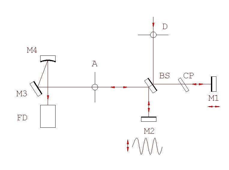
The basic optical configuration of the autocorrelator is similar to that of an
interferometer (Figure.1).
Figure 1.
An incoming pulse train is split into two beams of equal intensity. An
adjustable optical delay is inserted into one of the arms. The two beams are
then recombined within a nonlinear material (semiconductor) for two photon
absorption (TPA). The incident pulses directly generate a nonlinear TPA
photocurrent in the semiconductor, and the detection of this photocurrent as a
function of interferometer optical delay between the interacting pulses yields
the pulse autocorrelation function. The TPA process is polarization-independent
and non-phasematched, simplifying alignment.
The two beams propagate in a collinear fashion (interferometric configuration).
This configuration results in an autocorrelation signal that is on top of a
constant background.
This background is produced by TPA photocurrent resulting from the portions of
the scan during which the pulses are not overlapped.
The Reef RT autocorrelator has been specifically designed to measure the width
of pulses from femtosecond lasers. For the measurement of laser pulses the only
other item you need is an oscilloscope. Although not necessary, a storage
oscilloscope is convenient when operating in the interferometric mode since it
allows you to calibrate the display directly using the interference fringes that
make up the pulse envelope.
KEY COMPONENTS
The Reef RT autocorrelator consists of an opto-mechanical assembly and
electronics:
§ Beam Splitter
§ Scanning block with measuring converter
§ Variable Delay Line
§ Focusing Mirror
§ TPA-Detector with amplifier
§ Delay Sensor
§ Control Unit
SPECIFICATIONS
Pulse width - 10fs… to 6ps
Input pulse repetition rate - 10kHz to CW modelocked
Scan nonlinearity - <1%
Sensitivity (P-av P-peak) - <10(mW)2
Input polarization linear - horizontal (vertical specify with order)
Wavelength range: -700 - 1000nm
(1000 – 1400nm Optional)
Scan rate variable - 0,1 - 20Hz
Detection - diode with TPA
Electrical power choices - 100-110V(220V), 50-60 Hz
Dimension: - optical unit – 170mmx134mmx105mm
- control unit – 80mmx190mmx250mm
WARNING! LASER SAFETY
The protective housing of this product should always in place during normal
operation.
Removal of the protective housing may expose the user to unnecessary radiation,
and should
be done only in accordance with specific instructions given in this manual. Be
very careful
executing any step of alignment. Avoid any exposure to the direct and reflected
laser beams.
Direct and reflected laser radiation can cause serious eye damage. Remember,
that IR
radiation is invisible or looks like the red radiation from a low intensity He-Ne
laser.
However, it is dangerous even at lowest intensity. Even diffuse reflections are
hazardous.
Check all reflections and provide enclosures for beam paths whenever possible.
SAFTY CHECK LIST
§ Wear protective goggles whenever possible.
§ Please follow all safety instructions of your laser and use their
recommendations in your work.
§ Keep all beams below eye level always. Never look in the plane of
propagation of the beams.
§ When possible, maintain a high ambient light level in the laser operation
area.
§ Provide enclosures for beam paths whenever possible.
INSTALLATIONS AND ALIGNMENT
5.1 Reaching good alignment is easy if you use two external mirrors to direct
the
laser beam into the autocorrelator. Input power should be <20mW!
5.2 Install optical unit of the autocorrelator on the optical table horizontally
at
appropriate level. Use bottom screws to adjust level. Attach the unit to the
table using clamps.
5.3 The height of the autocorrelator can be changed relative to the optical
table.
5.4 The polarization of the laser input to the autocorrelator must be
horizontal.
(Vertical –optional).
5.5 Direct laser beam through the aperture A1 onto the centre of the mirror M2
(through beam splitter BS) (Figure.2). For visible beams, this alignment can
be done visually; for infrared beams, a viewer should be used.
5.6 Move the correlator to direct reflected beam (from M2) nearly back to the
center of the aperture A1 (The beam reflected exactly back can cause
feedback in the laser). The Autocorrelator has been aligned at factory. Under
careful transportation conditions you can try to continue alignment from 5.15.
5.7 Adjust beam splitter (BS) to direct beam (reflected from M2 and BS) to the
center of aperture A2.
5.8 Direct beam reflected from M1 to the center of A2 too. If the beam reflected
from the M2 propagates far from the center of A2 or M2, you should change
the direction of the input beam with external mirrors or turn autocorrelator as
a whole. Repeat the above mentioned procedure.
5.9 Remove M3 with holder.
5.10 Place white screen at 30 - 50 cm distance from the autocorrelator and watch
spots of light reflected from M1 and M2.
5.11 Adjust BS and M1 to reach coincidence of spots from two beams on the
screen.
5.12 Watch spot movement while adjusting mirror M1 with smooth stepping of the
micrometric screw (One step <=10mkm). Interferometric fringes will appear
when arms of the autocorrelator become equal. The picture should have
7
good contrast and no more than one interferometric maximum should be
watched.
5.13 Place M3 mount into the autocorrelator.
5.14 Adjust M3 to direct beam onto the sensitive area of photodiode (PD).
5.15 Connect optical unit to terminal “EXT” at rear panel of control unit.
5.16 For details we suggest you consult the Optical Delay Control Unit User
Manual
(see Appendix A).
5.17 Connect oscilloscope input to “Amplifier out” BNC connector of control
unit.
Synchronization could be performed from “Trig” signal (see Appendix A).
5.18 Make sure that no pump laser radiation propagates inside the autocorrelator.
5.19 Switch power on.
5.20 Set the control “Hi” – “Low” as follows: For 10….1000kHz input pulse
repetition rate (amplifiers) – “Low”; For >1000kHz input pulse repetition rate
(generators) – “Hi”. Push knobs “Amplifier” and “Generator” to select mode of
operation.
5.21 Set-up oscilloscope sensitivity - 100 mV/cm scale.
5.22 To adjust retro-reflector M2 oscillation amplitude and frequency, adjust
“Ampl.” and “Freq.” with the “Generator” knob. You should see
autocorrelation functions on the oscilloscope screen (50-100msec/div) like
Fig.3.
5.23 To maximize signal rotate focusing screw SF. (It may be necessary to reduce
intensity of the input light to keep the signal less than 10V).
5.24 Moving retro-reflector M1 with micrometric screw find position in the
middle
between two end positions (correlation functions disappear in the end
positions).
5.25 Find good position of the single autocorrelation function on oscilloscope
screen using “DELAY” control.
5.26 To display interferometric autocorrelation function (Figure.4) set low
frequency (“Freq” 2-5Hz) and big bandwidth (“Filter” -max). The
autocorrelation function must be symmetric. If the function is observed to be
asymmetric, the autocorrelator is either misaligned relative to the input beam
or internally misaligned.
8
L O N G R A N G E S C A N N I N G ( U P T O 6 P S )
5.27 The scanning range of the M2 is adjustable to 1mm which means a time
delay >6ps.
5.28 The electrical signal (“Sin”) is proportional to the mechanical position of
M2.
5.29 Use oscilloscope in X-Y mode to increase linearity.
----------------------------------------------------------------------------------------------
(Optional: The measuring converter of linear movements can be installed into
AA-10D. An
electronic copy signal (use out “DX”) exactly proportional to the mechanical
position of the
M2 allows one to operate the oscilloscope in X-Y mode. In this case linearity is
better than
1% over the whole scan).
DETERMINATION OF PULSE
DURATION
Move the distance calibrator until arrow is in the middle of scale. Attach
calibrator (MH)
to the optical plate using screw. Move M1 with screw (ST) and simultaneously
measure
change of distance with help of distance calibrator and displacement of
autocorrelation
function on the oscilloscope screen. Find two distances corresponding to
positions of
autocorrelation function at 1/2 of the maximum. Calculate the difference DL. You
can
measure the width (Dt) of autocorrelation function taking into account that 15mm
measuring
distance corresponds to 100 fs. To get pulse width (Dt) you should divide Dt by
1.41
assuming Gaussian pulse shape or divide by 1.55 assuming sech2 shape.
(Roughly Dt (fs) = DL (mkm) x 4).
In measuring a pulse that has a width corresponding to <30fs, it is important to
consider
possible sources of error. Due to the effect of group velocity dispersion within
the BS fused
silica plate 1mm-thick the measured pulse width to be broadened by <1fs. To keep
this
broadening at a minimum value compensation plate (CP) should be installed. To
minimize
dispersive effects only gold mirrors are employed.
References
1. E. P. Ippen and C. V. Shank, in Ultrashort Light Pulses, S.L.Shapiro, ed.
(Springer-Verlag, New York, 1977), pp.89-92.
2. J.-C. Diels and W. Rudolph, Ultrashort Laser Pulse Phenomena: Fundamentals,
Techniques, and Applications on a Femtosecond Time Scale (Academic, San Diego,
Calif., 1996), pp. 365-399.
3. J.-C. Diels, J. J. Fontaine, I. C. McMichael and F. Simoni, Appl. Opt. 24,
1270 (1985).
4. P. Heinz, A. Reuther, A. Lauberean, Optics Comms, 97, 35 (1993).
5. D.H. Auston, Appl. Phys. Letts, 18, 249 (1971).
6. W. Leupacher, A. Pezkofer, Appl Phys. B, 29, 263 (1982).
7. A. J. De Maria et al , IEEE, 57, No1, 2 (1969).
8. H. Schulz, H. Schuler, T. Engers and D. Von Der Linde, IEEE J.Quantum
Electron. 25, 2580 (1989).
9. J.-C. Diels, J. J. Fontaine and W. Rudolph, Revue Phys Appl., 22, 1605
(1987).
10. J. G. Fujimoto, A. M. Weiner and E. P. Ippen, Appl. Phys. Lett., 44(9),832
(1984).
11. J.K.Ranka, A.L.Gaeta, A.Baltuska, M.S.Pshenichnikov, D.A. Wiersma, Optics
Letters, 22, No.17, 1344 (1997).

Figure 3
Figure 4
Appendix A
G E N E R A L I N F O R M A T I O N
The Reef RT control unit is intended for driving moving mirror actuator and
sensing mechanical
mirror position.
Control unit consists of sine generator of variable frequency, variable gain
amplifier, output driver
and inductive position sensor (optional), see Figure. A1.
Output signal amplitude and frequency are controlled by an on board CPU.
Parameters are
stored and recalled in/from flash memory. Generator frequency is variable in a
range of 0.1...20 Hz
in 42 steps; output amplitude is variable in a range 0...+8V in 50 steps. . Two
front panel rotary
knobs labeled «Amplifier» and «Generator» control gain, bandwidth and output
sine frequency and
amplitude respectively. Red LED digital display shows actual v alue of amplitude
(0...50 in arbitrary
units) and frequency (0.1...20 in Hz). Output power driver can output up to +8 V
to 10 Ohm load
and is short-circuit protected.
Generator outputs are:
• «Sin» - fixed amplitude + 10V sine wave, BNC type connector, placed on a rear
panel.
• «Trig» - 12V amplitude logical signal. Its phase relative to output sine can
be adjusted by
• «Delay» potentiometer from a front panel.
Optional: Mechanical position sensor consists of 32 kHz generator driving fixed
coil and
synchronous detector, sensing sample signal. Output value +10 V at «DX»
connector corresponds to
+ 1 mm movement. Position sensor is static and can measure any steady mirror
shift.
Figure A1
E X T E R N A L C O N N E C T I O N S A N D O P E R A T I O N C O N T R O L
Check that power switch is set to off. Connect power cord to 100V 50-60Hz main
outlet. Connect
measurement equipment to output BNC connectors. Switch power on. Red display
shows current
values of a gain (or bandwidth) and frequency (or amplitude).
To adjust mirror oscillation amplitude, push “Generator” knob to set “Ampl” mode
and rotate the
knob. Right displayed value will change in a range of 0-50, corresponding to
about 0-8 V output
amplitude. Set value is immediately stored in a nonvolatile memory.
To adjust mirror oscillation frequency, push “Generator” knob to set «Freq» mode
and rotate the
knob. Right displayed value will change in a range of 0.1-20 Hz. Set value is
immediately stored in a
nonvolatile memory.
To adjust the gain of signal amplifier, push “Amplifier” knob to set the “Gain”
mode and rotate
the knob.
To adjust the bandwidth of amplifier, push “Amplifier” knob to set the “Filter”
mode and rotate
the knob.
Setting amplitude and frequency value; check mirror movement to not reach
position limits,
disturbing parasitic oscillations.
Synchronization could be performed either from «Trig», “Sin” or «DX» (optional)
signals.
Synchronization from first two signals is rather convenient in a case of large
mirror movement range,
but may be unstable due to mechanical vibrations of mirror elastic holder.
Synchronization from
«DX» signal avoids this error, but could be unstable in case of small
oscillation amplitude. The best
data acquisition method consists of PC-based 2-channel ADC board collecting data
array and
averaging them aft er acquisition.